The new version 7 release of Cresset’s workbench for ligand-based and structure-based modelling is packed with new and enhanced scientific features and methods, including enhanced sampling of hydration patterns with Grand Canonical Nonequilibrium Candidate Monte Carlo (GCNCMC¹) for molecular dynamics and Free Energy Perturbation (FEP) calculations, QM semi-empirical calculations, the new ensemble covalent docking method, and Consensus models for building predictive QSAR models.

This release also expands the choice of available tools to troubleshoot Flare FEP experiments, analyze dynamics trajectories, create ligand custom parameters for dynamics and FEP simulations, and prepare ligand structures for further studies.

Parallel processing and a new calculations window enable launching, running, and monitoring multiple jobs within the same Flare project; together making the platform more efficient, collaboration-friendly, and simpler to use.

More efficient water sampling and increased predictive performance for Flare FEP

More efficient water sampling with GCNCMC is available in Flare V7 for both molecular dynamics and FEP experiments. Combining traditional Grand Canonical Monte Carlo² (GCMC) with Nonequilibrium Candidate Monte Carlo (NCMC), this method performs water insertions and deletions in a gradual, nonequilibrium fashion, improving the sampling of hydration patterns into the protein active site.

Using GCNCMC during the equilibration stage of Flare FEP calculations can significantly boost the predictivity of the method, especially in protein-ligand complexes where the active site features occluded pockets, typically difficult to hydrate (Figure 1).

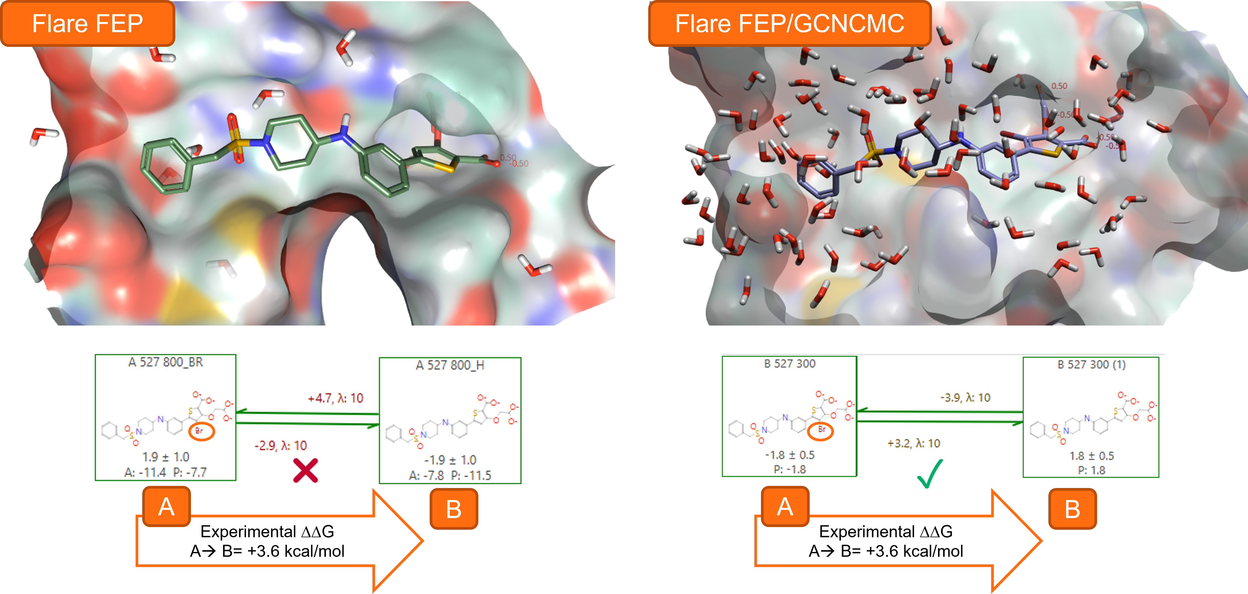
Figure 1. Using GCNCMC during the equilibration stage of Flare FEP calculations to transform ligand A (from PDB:2QBP, PTP1B Ki = 4 nM³) into ligand B (PTP1B Ki = 2000 nM³) significantly increases the accuracy of the FEP predictions.

Enhanced Flare FEP analysis tools

Sub-graph analysis is a new feature for the Activity Plot which further expands Flare’s choice of tools for analyzing the results of FEP benchmark experiments. These are routinely run at the beginning of a Flare FEP project to ensure that the system is set-up correctly, confirming the predictive ability of the method for the protein target/ligand series under investigation by comparing the experimental versus predicted ΔG for each ligand in the Activity Plot (Figure 2).

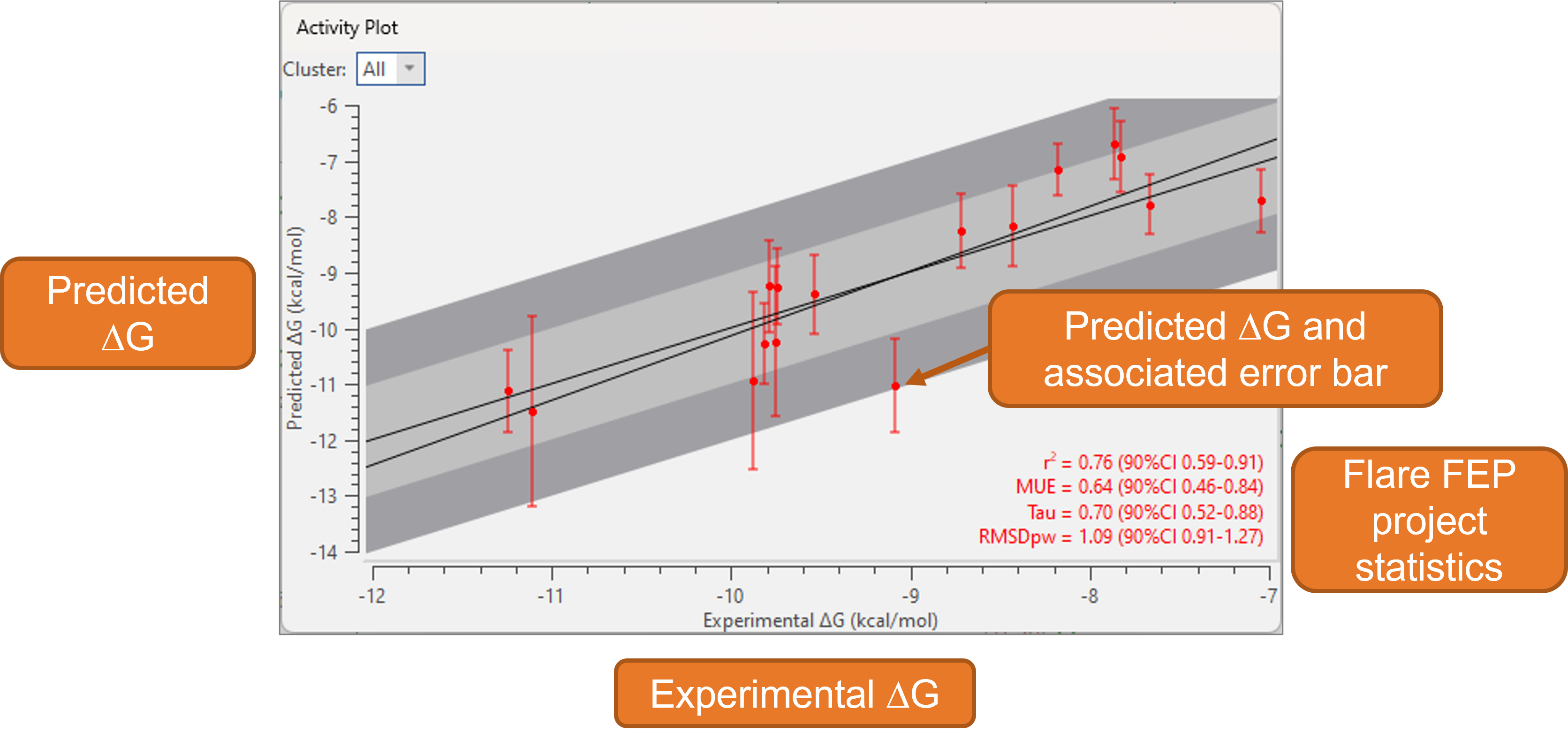
Figure 2. The Activity Plot for a Flare FEP project.

In the perturbation networks of Flare FEP projects ran on real drug discovery data, it is common to observe some granularity – small groups of highly congeneric, highly interconnected compounds. Relative ΔΔG predictions for the molecules in these groups are typically precise and reliable. However, if the connecting link(s) to the rest of the network are problematic, or if the network also includes compounds with less precise predictions, the statistics of entire dataset is affected, resulting into overestimated prediction errors for the compounds in the well-behaved groups, where the relative ΔΔG predictions can instead be totally trusted.

In these cases, sub-graph analysis can be useful to identify clusters of compounds with lower internal error statistics where predictions are more reliable and highlight problematic transformations that contribute to large statistical errors in the FEP project. For example, in the project in Figure 3 two clusters of compounds are found. The predictions for compounds in cluster #1 (purple) are less precise, as shown by the large error bars in the Activity Plot, as many links are affected by some degree of hysteresis. Predictions for the molecules in cluster #2 (green) are instead more precise (smaller error bars). As a result, we can highly trust the relative ΔΔG predictions for the molecules in #2, but not so much the predictions for molecules in #1, or between #1 and #2, as the connecting links also show hysteresis (orange ovals).

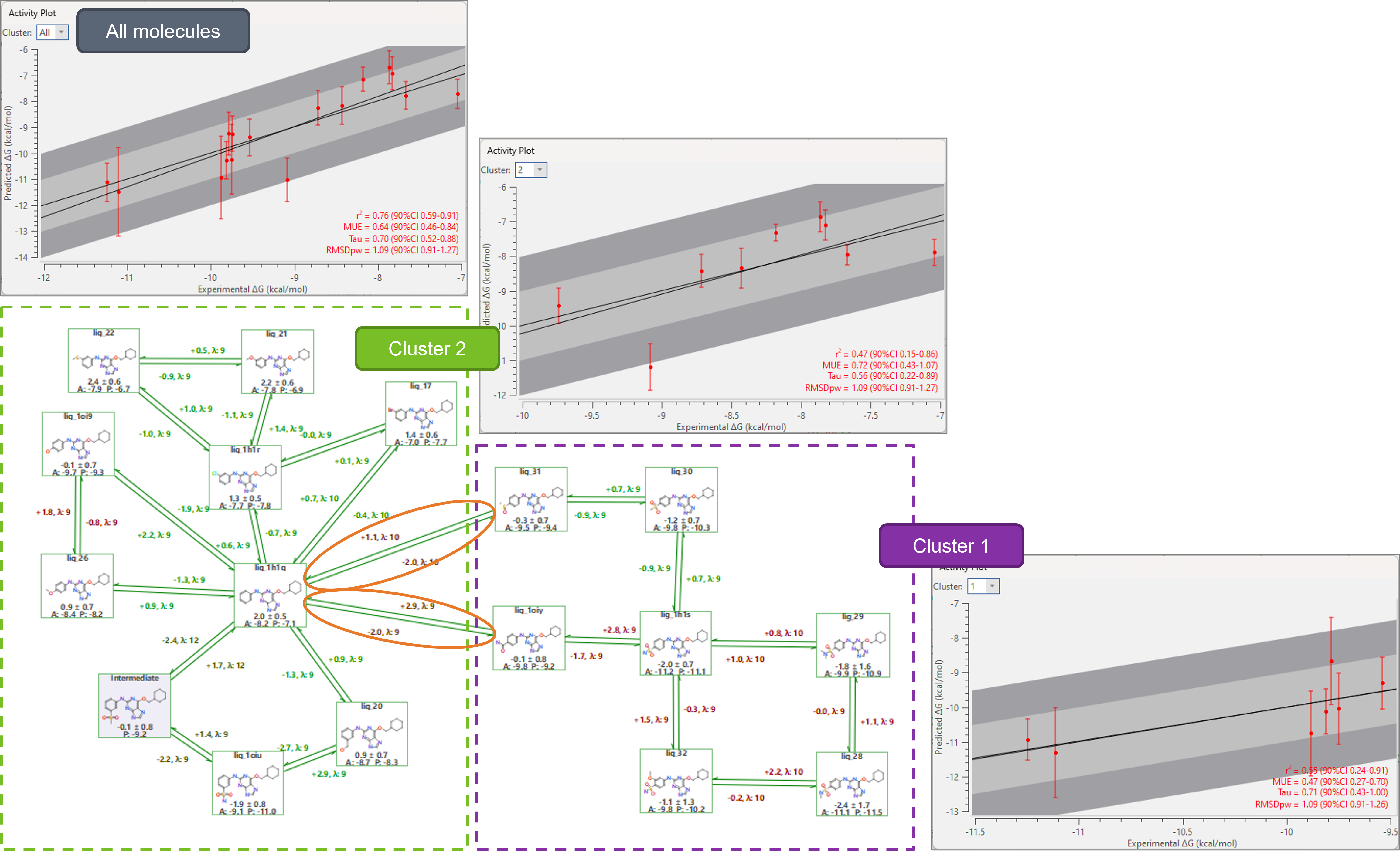
Figure 3. Sub-graph analysis in Flare V7 is useful to identify clusters of compounds with lower internal error statistics where predictions are more reliable and identify problematic transformations that contribute to large statistical errors in the FEP project.

Faster QM calculations with the new semi-empirical method

The new semi-empirical tight-binding method, based on the GFN2-xTB^4,5 implementation, further expands the choice of options for performing Quantum Mechanics (QM) calculations in Flare V7. Recommended for large ligands, this method can be used for both geometry optimization and single-point energy calculations with moderate accuracy. Furthermore, thanks to Flare’s flexible implementation, the computational efficiency of your QM workflow can be optimized by running fast semi-empirical minimizations followed by single-point energy refinement at DFT-level (Figure 4).

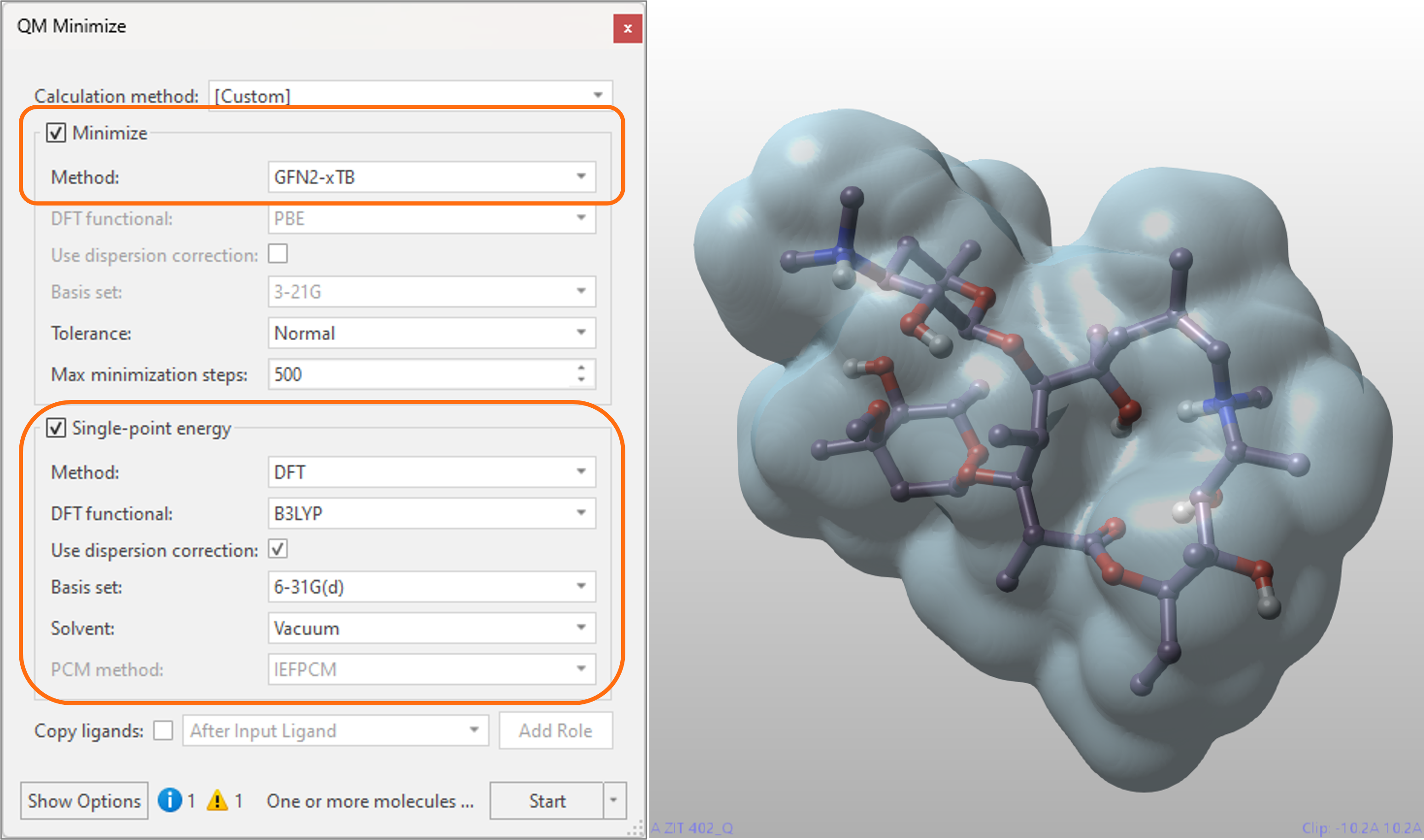
Figure 4. The geometry optimization at semi-empirical level of the macrolide Azithromycin, followed by a DFT-level single-point energy refinement in either vacuum or solvent, takes only a few minutes to complete on a laptop, enabling a computationally efficient workflow for larger ligands. Cyan surface = QM electron density.

pyflare users will also be able to access computationally efficient QM calculations from the command line with the new ‘qm.py’ script.

Enhanced molecular Dynamics with new analysis tools

For molecular dynamics experiments, the GCNCMC option can be activated either during the equilibration stage or over the whole duration of the simulation. This enables an enhanced sampling of the hydration patterns in the region of protein active site surrounding the ligand included in the simulation, and often leads to increased sampling of bound ligand conformations (Figure 5). Advanced options enable the fine-tuning of the GCNCMC sphere size and the move frequency.

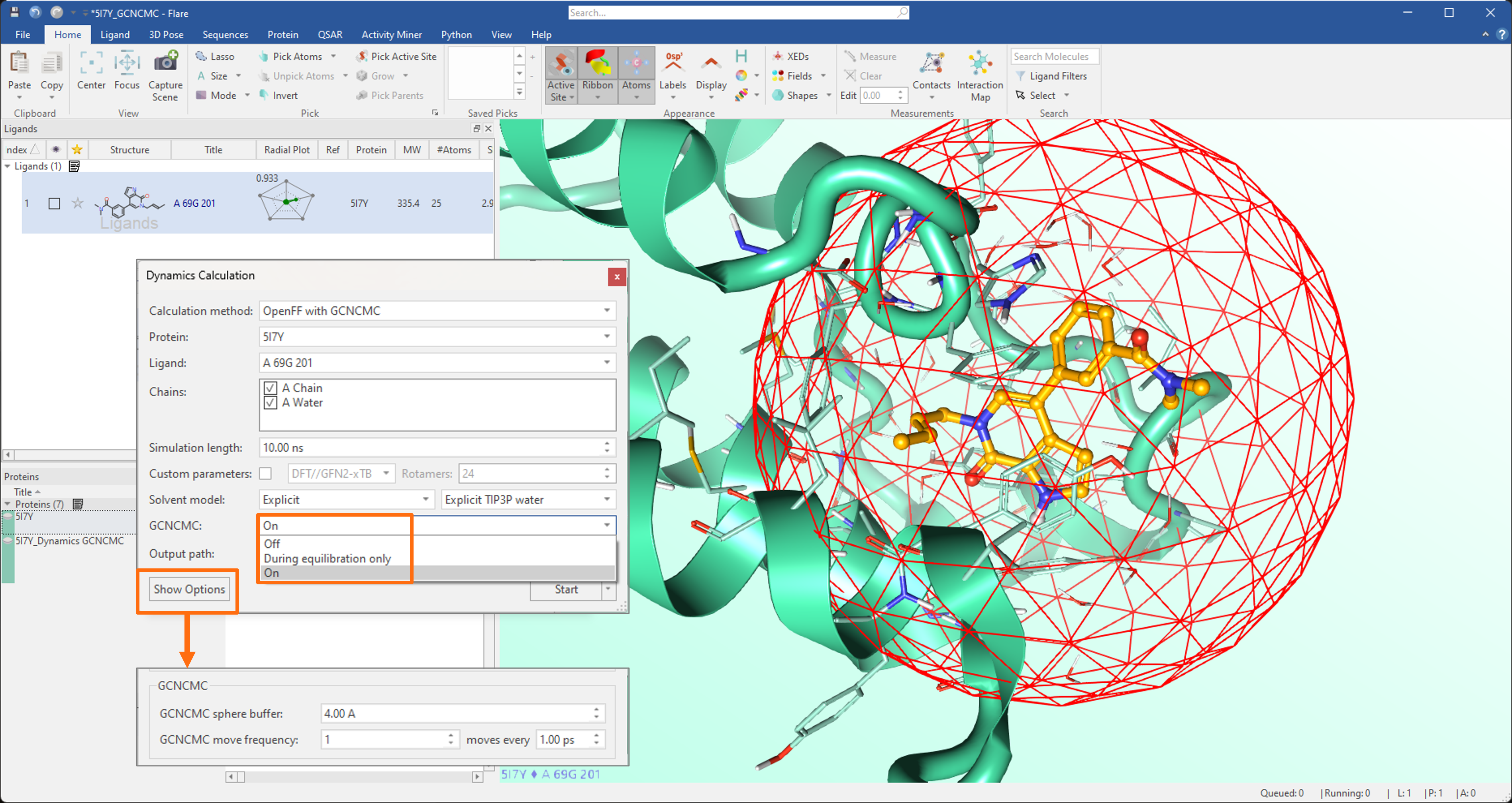
Figure 5. In molecular dynamics simulations, the GCNCMC option can be activated during the equilibration stage only or over the whole duration of the simulation.

The new ‘Export Trajectory’ button (Figure 6 - left) can be used to export the whole dynamics trajectory, or only the desired frame range, providing an efficient workflow for ‘trimming’ the trajectory to include only the frames in a range of interest. The trimmed trajectory can then be imported back into Flare, and associated to the protein it was exported from, by pressing the ‘Open Trajectory’ button (Figure 6 – right).

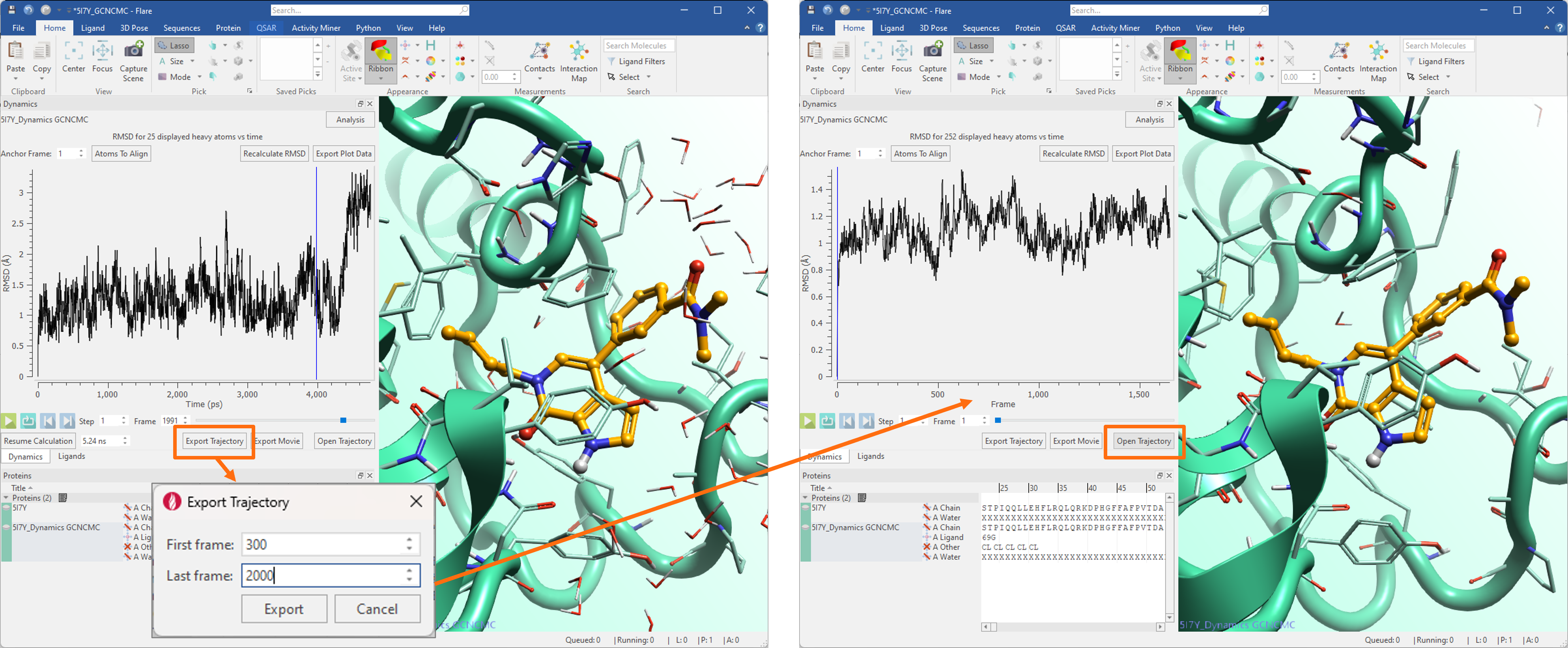
Figure 6. Left: the new ‘Export Trajectory’ button can be used to export either the whole dynamics trajectory, or only the frames in a range of interest. Right: the exported trajectory can then be imported back in Flare pressing the ‘Open Trajectory’ button.

Clustering of dynamics trajectories has also been enhanced with the capability to perform the analysis only on a selected range of frames.

New and enhanced methods for calculating accurate custom torsion force field parameters

Accurate torsion force field parameters are essential to reliably predict the thermodynamic properties of small molecule ligands and cofactors. In Flare V7 we have further expanded the choice of algorithms for creating optional custom torsion parameters in support of molecular dynamics and Flare FEP calculations, with the inclusion of the new hybrid DFT//GFN2-xTB method (Figure 7).

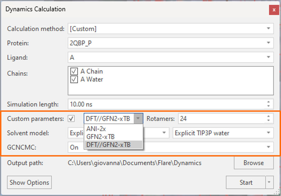
Figure 7. Flare V7 offers an expanded choice of algorithms for creating custom torsion parameters for the Open Force Field.

Strongly recommended for all small molecules (neutral and charged⁶), this method calculates DFT single-point energies at B3LYP-D3BJ/DZVP level on geometries obtained with the GFN2-xTB tight-binding semi-empirical method. In this way, good calculation performance is achieved thanks to the fast semi-empirical geometry optimization, while the ab-initio method is employed to perform high-quality energy calculations.

The existing ANI-2X⁷ and GFN2-xTB⁵ methods have also been updated with an enhanced fragmentation algorithm.

Enhanced QSAR capabilities to build predictive models

The new ‘Consensus’ regression and classification models join the existing panel of robust and well validated machine learning (ML) methods available in Flare (Figure 8). Running a Consensus regression model (Figure 8 – left) will cause Flare to run the Gaussian Process, MultiLayer Perceptron, Random Forest and Support Vector Machine models and predict the activity of compounds as the average of the predictions from each individual model. Consensus classification (Figure 8 – right) instead predicts the class/category of molecules as the class with the highest sum of predicted probability by the MultiLayer Perceptron and Random Forest classification models.

This creates a ‘consensus’ for the predictions, enabling you to prioritize the ligands which all the regression or classification models agree would be a good idea to make.

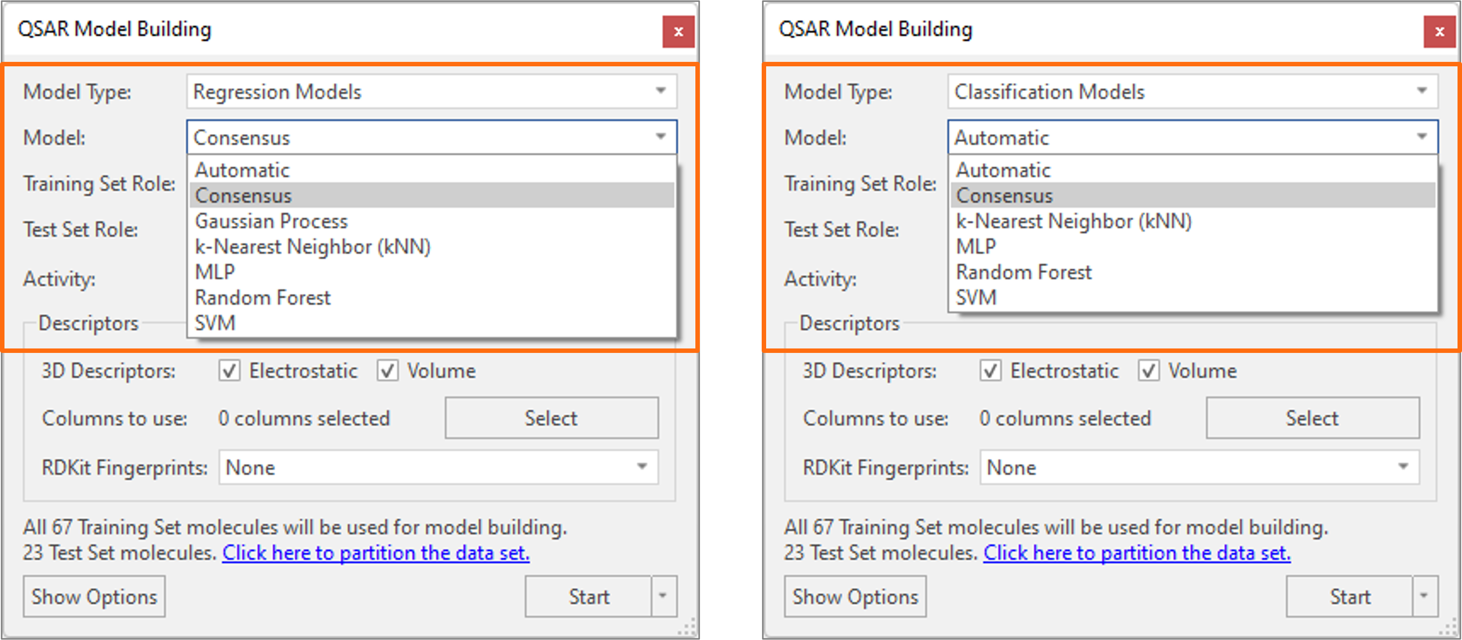
Figure 8. Consensus regression (left) and classification (right) models enable you to prioritize the ligands which all the machine learning regression or classification models agree would be a good idea to make.

In Flare V7, machine learning regression and classification models can be built seamlessly using a choice of different RDKit fingerprints⁸ (Figure 9 – left). Furthermore, several commonly used physico-chemical descriptors⁹ can be imported from the RDKit into the Ligands table using the Column & Activity Editor (Figure 9 - right) and used as an alternative to Cresset 3D descriptors of Electrostatic and Shape for building predictive QSAR models of activity and ADMET properties.

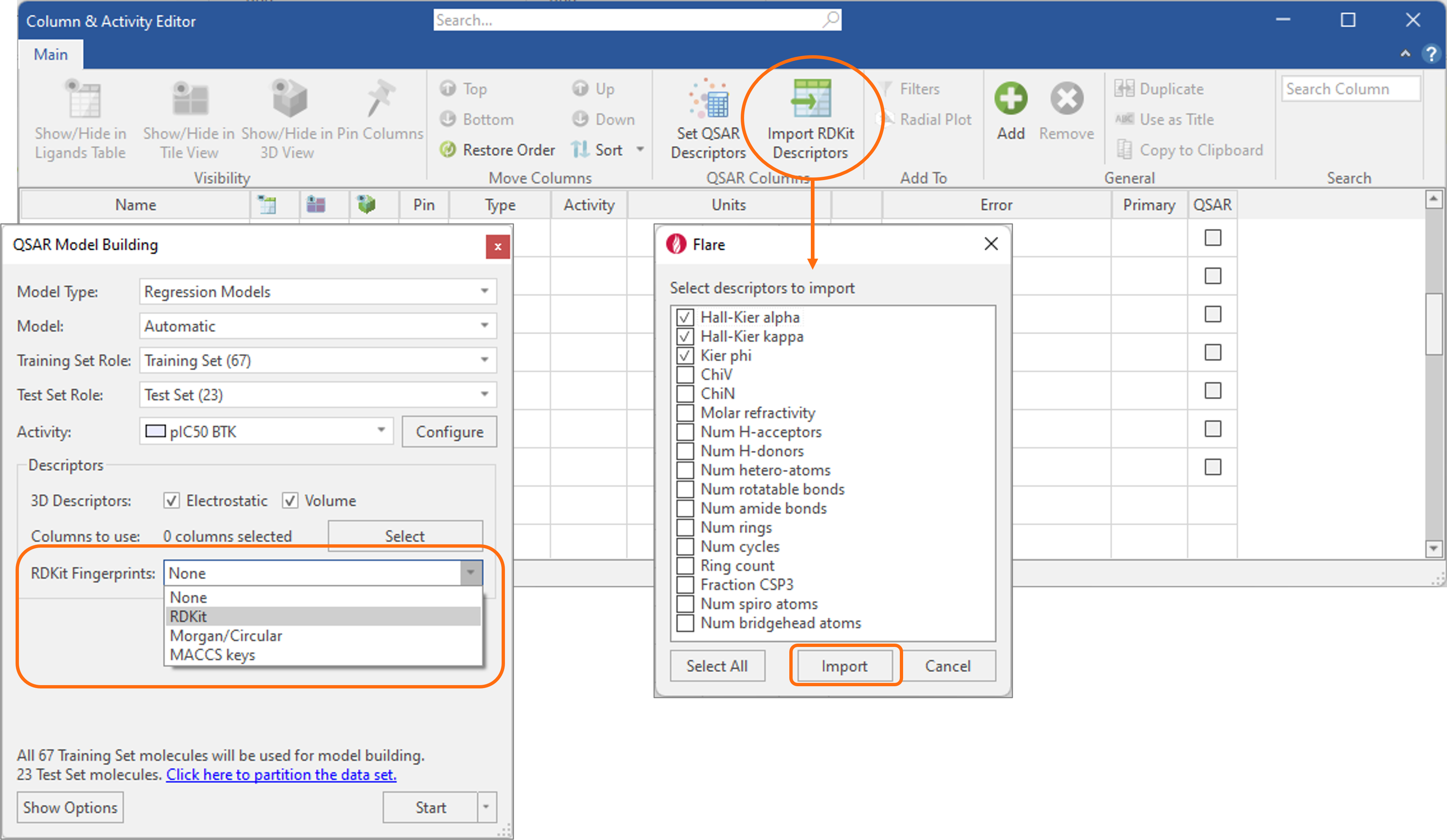
Figure 9. RDKit fingerprints and physico-chemical descriptors can be used in Flare to build predictive QSAR models of activity and ADMET properties.

Finally, Gaussian Process regression models now calculate standard deviation values for each predicted value, enabling you to gain confidence in the reliability of the predictions made by Flare before the compounds are synthesized and tested.

More options for docking and scoring

The new ‘Ensemble covalent’ method in Flare V7 merges together two popular docking methods: covalent docking, to generate sensible binding poses for covalently bound inhibitors, and ensemble docking for considering active site flexibility by including alternative active site conformations of the same protein in a single docking experiment.

As in covalent docking, the ligands to be docked must carry one of the many supported covalent warheads (more than 20): note that if the covalent warhead you want to use is not included, it can be easily added to Flare and shared with other colleagues (contact Cresset support for details). As in ensemble docking, the different protein conformations included in the study must be aligned together in 3D (Figure 10).

The docking grid (the region where the ligands will be docked) can be easily defined based on either the position of a known crystallographic ligand, or by manually picking appropriate protein atoms.

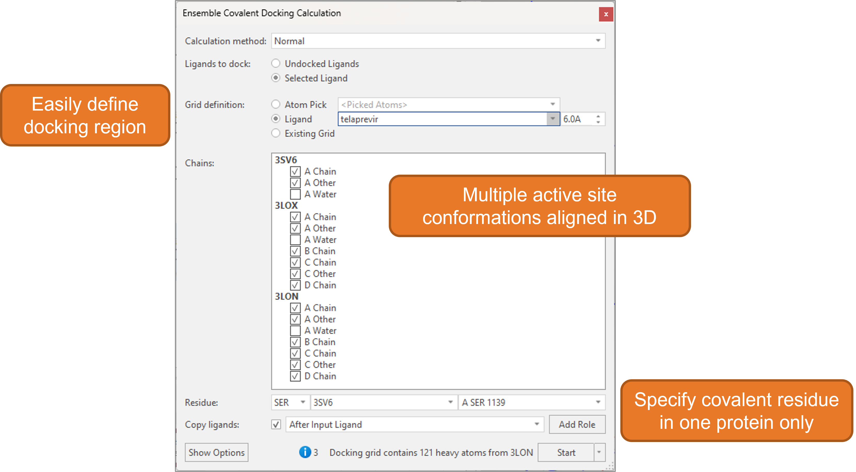
Figure 10. The calculation panel in Flare makes it easy to set up the ensemble covalent docking experiment.

It is sufficient to define the covalent residue in only one of the proteins: equivalent covalent residues in the other superimposed protein structures are automatically detected by Flare. Alternatively, it is also possible to manually pick individual covalent residues from each protein.

At the end of the ensemble covalent docking experiment, the binding poses generated by Flare’s covalent docking algorithm will be saved in the Ligands table associated to the protein they were docked into. The poses with the lowest Rank Score have the highest likelihood of reproducing the correct crystallographic pose (Figure 11).

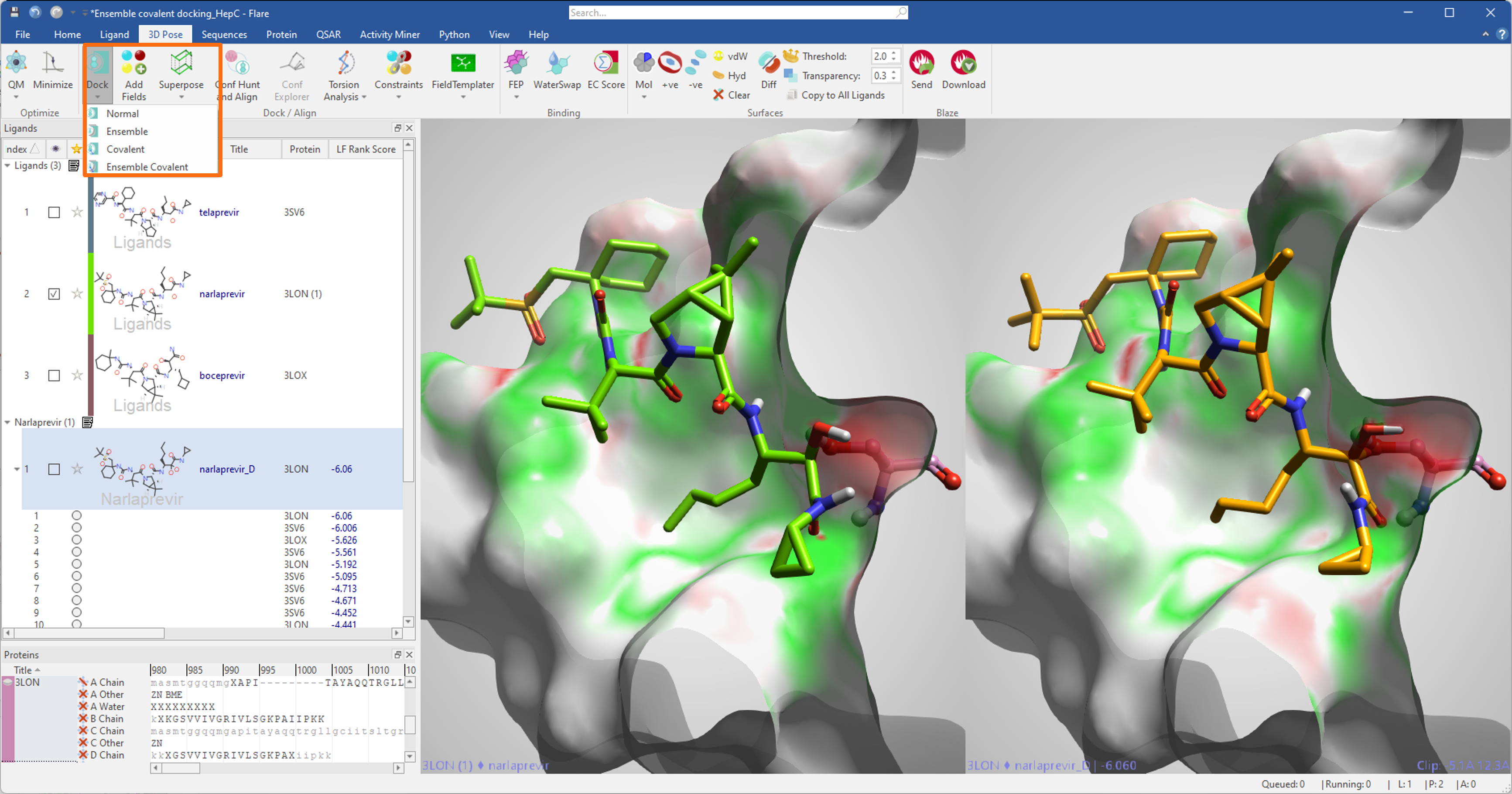
Figure 11. Results on an ensemble covalent docking experiment on covalent inhibitors of the HCV  NS3/4A protease complex. The 2D structure of narlaprevir was used in an ensemble covalent docking experiment performed on three different conformations of the HCV NS3/4A protease (PDBs 3SV6, 3LON, 3LOX). The top scoring pose found by Flare (right, in orange) closely reproduces the crystallographic pose for narlaprevir in PDB: 3LON (left, green). The protein surface is colored by Electrostatic Complementarity towards crystallographic (left) and docked (right) narlaprevir (green = good electrostatic complementarity; red = electrostatic clash).

In Flare V7 you will also find new, useful advanced options for your docking experiments. A new advanced option for covalent docking enables you to specify the warhead to use for your experiment by typing its SMARTS definition. This is useful in those cases where the ligands you want to dock carry more than one potential covalent warhead, and you want to use your knowledge of the chemical series under investigation to control the reacting group.

Another new advanced option for all docking methods in Flare enables you to specify which H-bond donor protein residues in the active site (choosing from each or all of Serine, Threonine, Tyrosine and Lysine) are allowed to rotate during the docking experiment. This provides an additional way of allowing side chain flexibility in your docking experiment and achieving optimal interactions with the protein active site.

Parallel processing

We have significantly enhanced the efficiency of calculations in this release by enabling Flare to run multiple jobs in parallel (Figure 12).

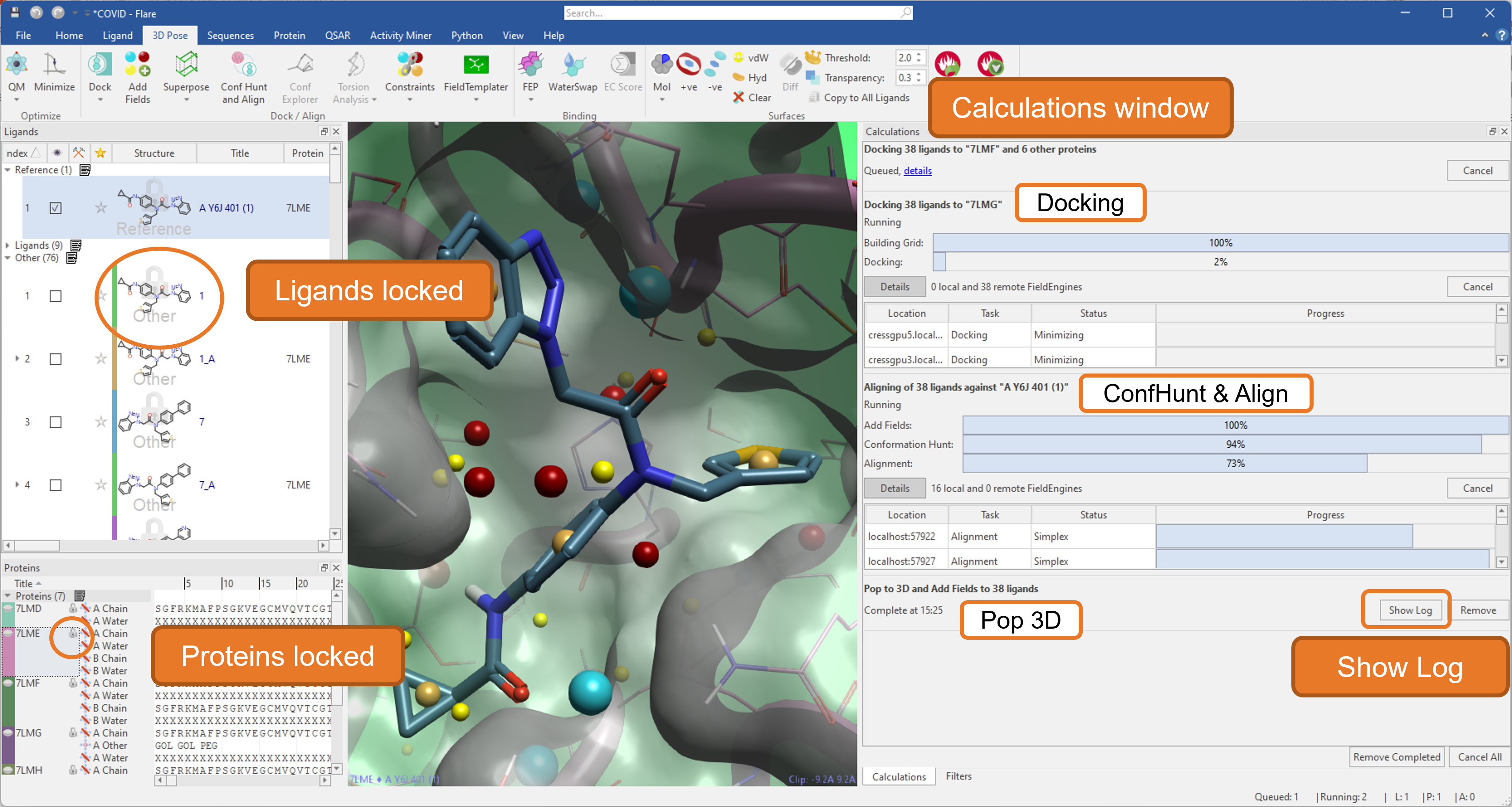
Figure 12. Running multiple jobs in parallel in Flare.

An intelligent locking system prevents the unintentional deletion or modification of ligands and proteins used in running jobs until they are finished. Furthermore, a re-designed calculations window monitors all running, queued, and finished jobs, giving easy access to the Log for each calculation.

Enhanced ligand preparation

The Ligand Prep function in this release is enriched by a new option to enumerate tautomers. Based on Cresset rules, tautomer enumeration gives you the choice to enumerate only canonical tautomers, as well as tautomers which are from highly likely to less likely in aqueous solution (Figure 13).

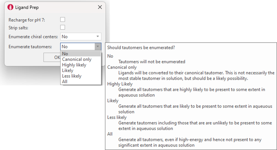
Figure 13. The new tautomer enumeration option for ligand preparation.

Creating biological assemblies during protein preparation

The functional form for many proteins in nature is that of a biological assembly, i.e. a macromolecular assembly of one or more units: for example, the functional form of hemoglobin has four chains. Importing biological assemblies in Flare was always possible, but in some cases required some manual intervention. In Flare V7, we added a new option to protein preparation to make it easy to import biological assemblies as described in the input PDB in an automated manner.

In Figure 14, on the left side, we can see PDB:6TOH (crystal structure of CCT365386¹⁰ bound to BCL6, a potential therapeutic target for the treatment of diffuse large B-cell lymphoma) after protein preparation in default conditions. On the right side, we can see PDB:6TOH imported using the ‘Create biological assembly’ option. The functional dimeric structure of BCL6 has been automatically imported and an important water-filled pocket in the binding site is now clearly visible.

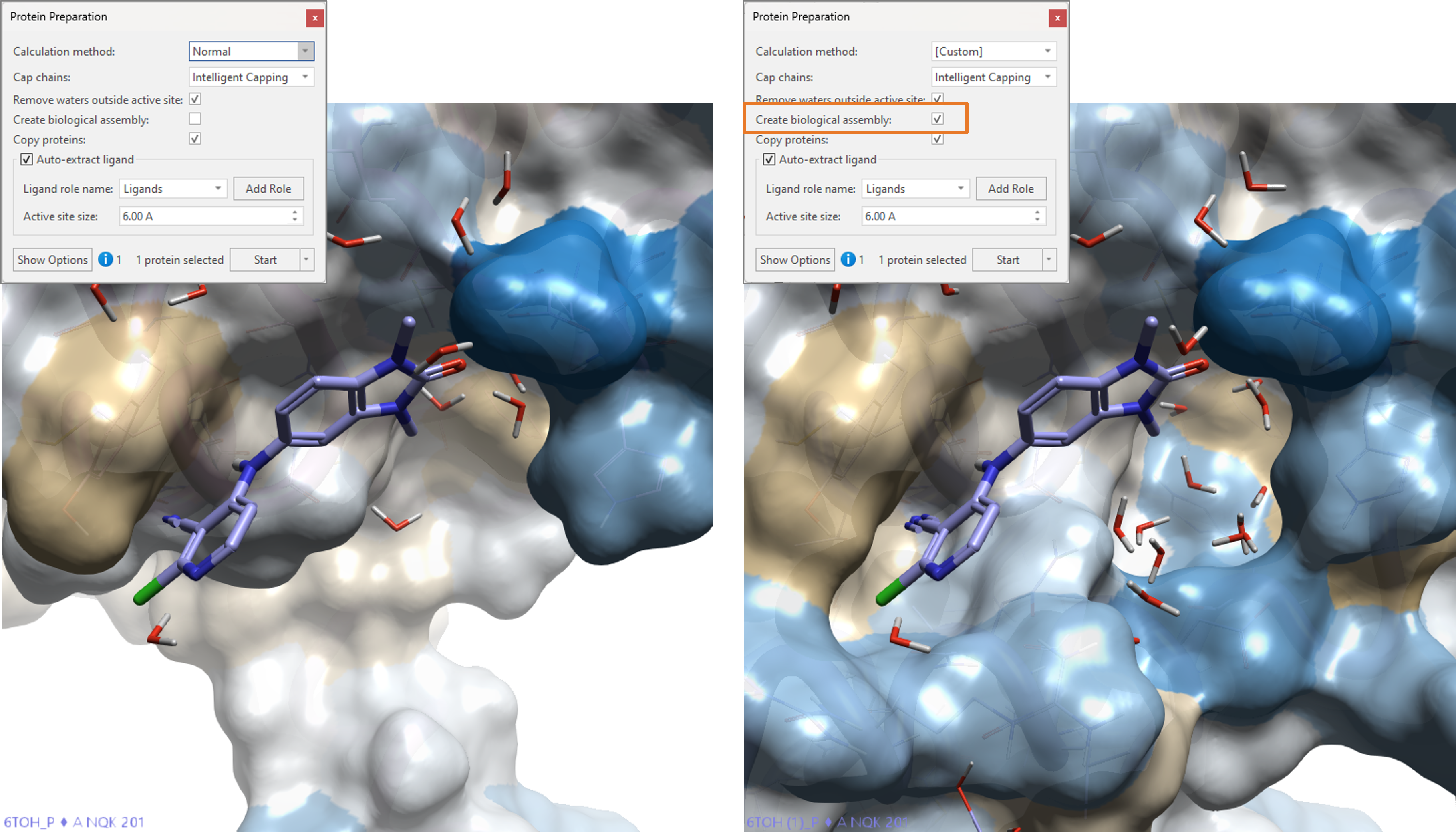
Figure 14. PDB: 6TOH imported and prepared in Flare using default conditions (left) and using the ‘Create biological assembly’ option (right) to automatically re-create the functional dimeric form of BCL6. The surface of the active site is colored according to hydrophobicity¹¹.

Other enhancements and improvements

New enhancements and improvements in Flare V7 also include:

• The ability to organize the Proteins and Alignment tables with roles
• Enhanced protein modelling:
  • The ability to build peptides and grow proteins in the editor
  • ‘Copy/Paste Loop’ functions to fix gaps in the protein of interest by copying loops from a different protein structure
  • The ability to insert a sequence of residues in the desired position
  • Functions for residues in the protein sequence with no 3D coordinates, enabling their selection, deletion, placement into new chains, and chain splitting
  • The workflow for single-point mutations now gives the choice to prepare only the mutated residues or the whole protein
    An interactive sequence ruler bar in the Proteins and Alignment tables, to highlight/select all residues in the same position across all proteins
• Enhanced library enumeration, with clearer naming and expanded definitions for reactions, as well as options for exporting/importing structure filters
• A new interface to the Mogul torsion analysis method (requires a valid CSD license)
• A new ‘Search’ box at the top of the Flare GUI, to quickly locate desired the Flare functionality such as ribbon tab buttons, menu items, and dockable windows
• A new function to export a Spin/Rock Movie
• Interactive Radial Plots
• AND/OR logic for filtering ligands based on their Tags
• An expanded choice of substituents for Hit Expander
• Enhanced visualization of R-Group Analysis results
• Existing scenes in the Storyboard can now be updated
• New permanent annotation of ligand titles for scatter plots.

Flexible software licensing for computational chemists, medicinal chemists, and academics

Whether you are interested in ligand-based or structure-based methods, or both, Flare features flexible licensing options to suit computational chemists, medicinal chemists, and academics. If you’d like to try Flare V7 on your projects, you can request an evaluation, today.

As part of the evaluation process, you’ll receive full support in installing the platform and accessing its wide range of features, while having the freedom to publish any results produced and use these for further research.