Background

Assessing the binding potency of millions of different compounds against a common protein target presents many challenges in a wet laboratory. Even with advanced lab robotics and automation platforms, wet laboratory high-throughput screening (HTS) is still hindered by time, resources, and finance.

As such, it is now commonplace to first consult structure-based drug design (SBDD) software platforms in attempt to filter out any compounds that are predicted to have low binding potency against the target of interest. This, in turn, frees up time, resources and finance as subsequent wet laboratory screening is only considering compounds we believe to have most promise.

Flare™ is a drug-design software platform which can be used to predict whether compounds will bind to a given protein target, using techniques such as molecular docking and Electrostatic Complementarity™ (EC) analysis which compares the electrostatics of the bound putative ligand with the binding site of the target protein. The Flare GUI can seamlessly run such calculations on a maximum of 10,000 ligands, but what happens when we have millions of ligands? In such a case, it would not be possible to store all these structures and run calculations within the GUI. This is where using the pyflarecommand line can be very useful.

pyflareis a dedicated Python binary that gives you access to Flare functionalities from within a command line Python script. This is incredibly powerful as it enables Flare calculations, such as docking and EC, to be executed on a command line interface on your dedicated computing cluster without the need to load and store molecules and proteins within the GUI. With the GUI capacity limitation lifted, this leaves us free to perform Flare calculations on much larger compound libraries.

This article will talk you through how we can write a pyflare  script to execute a docking and EC hit identification workflow. The real benefit of such a pyflarescript is the transferability: the script can be executed on the different drug discovery targets or compound libraries without being altered. To launch this workflow, all that you need are three files: your protein target stored as a PDB file, the associated crystallographic ligand stored as an SDF file, and the compounds you wish to test in your computational HTS also stored within a single SDF file.

So, let’s look at what such a hit identification workflow looks like when encoded into apyflarescript.

Initializing the project

The first thing we need to do is to create a new, blank, Flare project.

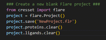
Figure 1. Creating a new Flare project using pyflare.

In the example shown in Figure 1, the Flare software library is first imported, giving us access to Flare’s calculation methods; a Flare project is then created and assigned to the variable ‘project’. By assigning the Flare project to a variable, it allows the user to perform operations such as saving your progress (i.e., using Python to perform ‘File > Save As’), clearing the current project data (i.e., using Python to perform ‘File > New Project’) as well as reading in and exporting structure files.

Loading protein and crystallographic ligand data

Now we have created a new Flare project, let’s begin by loading our prepared protein and crystallographic ligand into the project. These structure files are located in the working directory where we are executing thispyflarescript.

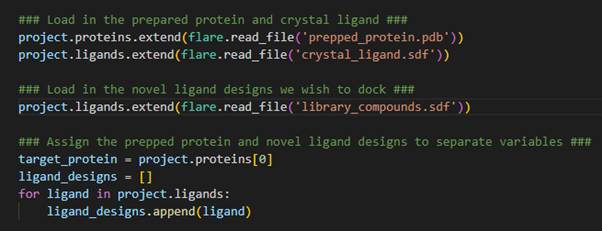
Figure 2. Loading protein and ligands into a Flare project.

The proteins.extend()and ligands.extend() operations enable us to load our prepared protein target and crystallographic ligand into the Flare project. Conceptually, we are ‘extending’ the current ligand and protein tables through the addition of these new structures. As these new structures are stored within separate files, we need to tell Flare to read these files using the ‘flare.read_file()’ command. The exact same procedure is also done for the SDF file encompassing our compound library.

Now that all the necessary structures for our hit identification workflow have been loaded into the Flare project, we now assign the target protein and library compounds to separate variables to be used in subsequent calculations. In this example, we only have a single protein loaded into our Flare project, which occupies the first data entry in the proteins table. As such, we can assign it the variable target_protein by calling the zero-index (1st entry) of the proteins table. For docking and EC calculations in pyflare, the ligands to be used in the calculation must be stored within a list format. Therefore, by creating the ligand_designs variable as an empty list, we can then use a for-loop to iterate through all the ligands loaded into the Flare project, assigning each to the ligand_designs list variable. The ligands are now stored in the correct format for calculation.

Preparing ligands for docking

The next stage in our hit identification workflow is to ensure all our ligand designs have adopted a minimum energy 3D conformation prior to docking. This can be done by performing a pop-to-3D calculation followed by a minimization calculation (Figure 3).

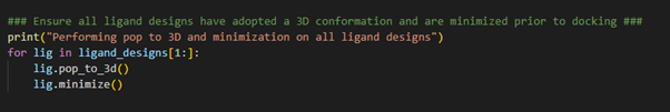
Figure 3. Pop-to-3D and minimization of ligand structures to be docked.

By establishing a for-loop, we can loop through all the ligands designs we have stored in the ligand_designs list variable and execute the pop-to-3D and minimize methods to obtain a low energy 3D conformation for each ligand design. Note the use of ligand_designs[1:], which allows us to skip the first entry within the ligand_designs list variable. Recall, the crystallographic ligand is the first entry within the ligand_designs list variable and therefore does not need converting to 3D.

The docking experiment

Now the ligand designs have adopted a low energy 3D conformation, we are at the right stage to carry out the first of our HTS experiments: docking (Figure 4).

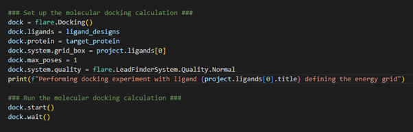
Figure 4. Setting up the docking experiment where our input ligands will be docked into the target protein.

We first initialize the docking operation through loading the docking class using flare.Docking(). We specify which ligands we wish to dock (e.g., our ligand_designs defined above), and which protein we wish to dock into. When configuring a docking calculation in Flare, we also need to be sure to define the energy grid box. This should be defined to encompass the target protein active site and, as such, can be designated as a region of 3D space that hosts the crystallographic ligand. This was the first ligand we loaded into the Flare project and, therefore, occupies the zero-index (1st entry) within the ligands table. In our example, we are only interested in storing the most stable binding pose for each ligand, which is achieved by setting max_poses to 1. We can customize the docking calculation quality by loading a defined pre-set tolerance. In our case, we have chosen ‘Normal’ tolerances. We can now start the docking calculation and wait for the result.

Calculating the EC for the docked poses

Once the docking is complete, the next stage is to calculate the EC score for each of the docked poses.

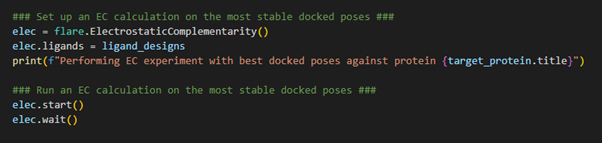
Figure 5. Calculating the Electrostatic Complementarity of the docked poses against the target.

After completion of the docking calculation, each ligand within the Flare project is now being stored in its most stable docked pose and is associated with the protein target. Therefore, upon initializing the EC calculation, through loading the Electrostatic Complementarity class using flare.ElectrostaticComplementarity(), we simply need to direct Flare in the direction of the ligand_designs variable which holds all the relevant information necessary to execute an EC calculation. We can now launch the EC calculation and wait for the result.

Triaging the results

The final step in the workflow is to determine which ligands show promise as good binders to the protein target. This is achieved by triaging the compound library by means of the docking and EC scores. Explicitly, we are interested in triaging based on the LF Rank Score (calculated during the docking experiment) and the EC Score (calculated during the EC experiment). A molecule with a good LF Rank Score and EC score could potentially be a strong binder to the target, and these are the ligands we wish to isolate from our dataset.

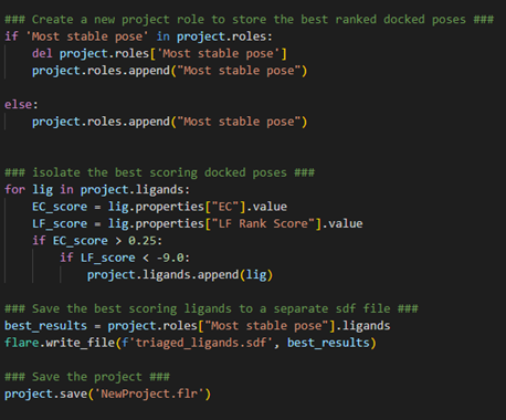
Figure 6. Analyzing and extracting the best-scoring result.

Firstly, let’s create a new project role, aptly named Most stable pose, to store the triaged ligands. We can first check whether such a role has been created before, and if so, delete and create it again. Otherwise, just create the role as normal using project.roles.append(). Now, for all the ligands in our project, we wish to identify the ligands with good EC scores (> 0.25) and good LF Rank Scores (< -9.00). Notice how we have used a nested if-statement here to ensure we are capturing ligands that satisfy both triage criteria. For each ligand we identify in our project that satisfies these criteria, we can store it in the Most stable pose role created above.

Finally, we can export our triaged ligands to a separate SDF file using flare.write_file() and save the project in case we wish to come back to it later.

Conclusions

In this article, we have executed a hit identification workflow, scripted in Python using thepyflarebinary, which has performed a computational HTS on a very large compound library and identified which ligands show promise as good binders to a target protein. This was all done without the need to load and store structures in the GUI. This workflow is completely automated, computationally fast, and does not suffer from GUI (data) storage limitations and is all made possible by the Python extension to Flare.

Request a free evaluation of Flare today to further explore its full portfolio of molecular modelling capabilities.